Update: I have moved the details of this strategy to edgeGiant.com. All further updates will be made there.
B y now, Joel Greenblatt has become a household name in the world of value investing. Greenblatt is the manager of Gotham Asset Management LLC, which he started in 1985 (as Gotham Capital) as a fund with a deep value philosophy. His book, The Little Book that Beats the Market, introduced to his audience a strategy for stock selection that focuses on companies that are both “cheap” and “good”. And while his book is certainly not big, it did give detailed instructions on how we can go about replicating his strategy, which in essence is a two factor long only model of stock selection.
"Cheap" and "Good"
Greenblatt defines "Cheap" as the value of a company relative to its earnings. Most often, we may see this represented as a ratio of the price of a security relative to its earnings (P/E). However, Greenblatt prefers to look at the ratio of pre-tax operating earnings as it relates to Enterprise Value (a measure of a company's equity value with its debt, excluding any cash it has on hand). This allows for companies with varying debt and tax structures to be more easily compared.
"Good" is represented by the Return on Capital of a company. This is described as the ratio of pre-tax operating earnings to the sum of a company's New Working Capital and it's Net Fixed Assets. In other words, Greenblatt is quantifying the amount of tangible capital required to operate a business, and seeing how much money each dollar of deployed capital will yield back.
In this series, we will take a closer look at the theory behind the Magic Formula and try to backtest and replicate the strategy programmatically. We will refrain from espousing on the merits of his two factor system, and instead focus on the details of the calculations involved, with the aim to match the Magic Formula methodology as closely as possible. To get started, let's first go through the formula as it is explained in the book:
The Formula
- Establish a minimum market capitalization (usually greater than $50 million).
- Exclude utility and financial stocks.
- Exclude foreign companies (ADRs)
- Determine company’s earnings yield = EBIT/ EV
- Determine company’s return on capital = EBIT/ (Net Fixed Assets + Working Capital).
- Rank all companies above chosen market capitalization by highest earnings yield and highest return on capital (ranked as percentages)
- Invest in 20 to 30 highest ranked companies, accumulating 2 - 3 positions per month over a 12 month period
- Rebalance the portfolio once per year, selling losers one week before the year and winners one week after the year.
- Continue over a long term period (5 to 10+ years)
Data
Our first consideration is a data source for company fundamentals. There are a number of data providers that can satisfy this need. An earlier version of this post used a license from Sharadar Core US Equities Bundle found on the financial data site Quandl. As of this publication, the price of this data package starts at $70 a month.
Since the time of the original post, we have pivoted to the data provided by Quantopian. Quantopian offers access to comprehensive Fundamentals coverage through their licence with both Morningstar and Factset, and we found these sources to be more robust (and Free) and easy to work with (and FREE) relative to the Sharadar data. There are, however, some downsides to using Quantopian, the biggest of which is that you are only allowed to access this data within their research environment, to prevent abuse and mass download of their valuable data sources. This can limit the complexity of the strategies, but should work just fine for Factor Modeling.
Getting Started
Quantopian offers a research environment where we can test ideas out interactively through a Jupyter
Notebook. From there, one can implement and backtest the idea through the IDE provided. The bulk of
the work will done using the pandas library in Python, in conjunction with a number of
quantopian specific modules. As with anything else, we get started by importing the
needed libraries. For the sake of this demonstration, I assume the audience is somewhat familiar with
Python and pandas, or have the requisite knowledge to find answers online via resources like
StackOverflow. To import the general modules, we start with:
import pandas as pd
import numpy as np
And then the specific quantopian modules we need:
from quantopian.pipeline import CustomFactor, Pipeline
from quantopian.pipeline.data.factset import Fundamentals as FFundamentals
from quantopian.pipeline.filters import default_us_equity_universe_mask
from quantopian.pipeline.data.morningstar import Fundamentals
from quantopian.pipeline.classifiers.morningstar import Sector
from quantopian.pipeline.domain import US_EQUITIES
from quantopian.pipeline.data.builtin import USEquityPricing
from quantopian.research import run_pipeline
In handling large datasets, especially as it relates to screening, Quantopian uses something called
a Pipeline API to facilitate fast computation. Specifically, Pipeline makes
it easier to find values at a point in time of an asset (Factor), reduce a set of assets into a subset for further
computation based on some evaluation (Filter), and group an asset based on properties that may
facilitate your desired screen (Classify). Combined, factors, filters, and classifiers represent a set
of functions that will get us a list of magic formula stocks at a given period in time. We'll do this
by creating a make_pipeline() function.
Step One
The first step in the Magic Formula dictates that we establish a minimum market capitalization (usually greater
than $50 Million). We will use Morningstar's calculation of market cap through Fundamentals.market_cap,
and qualify that it is at a date we specify by adding the method latest to the end of the object.
market_cap_filter = Fundamentals.market_cap.latest > 200000000
Step Two
Next, we make use of Morningstar's Sector Classification to exclude Financial and Utility companies.
sector = Sector()
sector_filter = sector.element_of([
    101, #Materials
    102, #Consumer Discretionary
    #103, #Financial
    104, #Real Estate
    205, #Consumer Staples
    206, #Healthcare
    #207, #Utilities
    308, #Telecoms
    309, #Energy
    310, #Industrials
    311, #Technology
])
Step Three
Step Three of the magic formula requires that we exclude ADRs, for similar reasons as Step Two in that
we cannot be sure of the capital structure of international companies and may not be comparing apples
to apples when determining things like EBIT or Rates of Capitalization. To do this, we leverage a
pre-screened list of securities in Quantopian called default_us_equity_universe_mask().
This base filter requires that the security be the primary share class for its company. In addition, the security
must not be an ADR or an OTC traded symbol. The security must not be for a limited partnership, and it must
have a non-zero volume and price for the previous trading day. The mask also has a parameter to
pass in a value for minimum market cap, which we'll again set to 200MM.
tradable_filter = default_us_equity_universe_mask(minimum_market_cap=2000000)
We then combine the filters to retrieve our stock universe.
universe = market_cap_filter & sector_filter & tradable_filter
Step Four
The fourth step of the magic formula is determining Earning's Yield, defined as EBIT/EV. Greenblatt uses a trailing twelve month EBIT, which differs from Morningstar's default fundamental EBIT value that only looks at the most recent quarter. One way to do this is to write a windowing function to aggregate quarterly values for the past four quarters. Alternatively, Quantopian's FactSet data has many of the data in a trailing twelve month basis, so we can switch to this for this part of our screen. **Note: FactSet Data on Quantopian contains a one year holdout period, so your backtest can only run up to one year prior to present day. For example, if you are working on this script on October 1st, 2020, then your backtest can only run up until October 1st, 2019. Not super ideal, and it makes the Morningstar Fundamentals a much more attractive solution if your intention is to find a list of suitable symbols for investment.
ebit_ltm = FFundamentals.ebit_oper_ltm.latest
ev = Fundamentals.enterprise_value.latest
earnings_yield = ebit_ltm/ev
Step Five
Greenblatt's return on capital differs from a typical ROE or ROIC value. Within the Magic Formula, a company's return on capital is measured as EBIT/ tangible capital employed. In other words, we're trying to find the tangible costs to the business in generating the reported earnings within the period, where tangible capital employed is more precisely defined as Net Working Capital plus Net Fixed Assets.
Net Working Capital is simply the total current assets minus current liabilites, with an adjustment to remove short term interest bearing debt from current liabilites, and another to remove excess cash. Greenblatt does not offer details on how excess cash should be considered, but it is often calculated based off of a percentage of cash needed relative to sales generated within a period. For our simulation, we'll take the Max(Total Cash - Sales_LTM * 0.03, 0)
Net Fixed Assets is then added back to Net Working Capital, in the form of Net PPE.
ppe_net = FFundamentals.ppe_net.latest
sales_ltm = FFundamentals.sales_ltm.latest
total_assets = Fundamentals.total_assets.latest
current_liabilities = Fundamentals.current_liabilities.latest
goodwill_and_intangibles = Fundamentals.goodwill_and_other_intangible_assets.latest
#cash = Fundamentals.cash_and_cash_equivalents.latest
cash = Fundamentals.cash.latest
excess_cash = max((cash-(sales_ltm*0.03)),0)
current_notes_payable = Fundamentals.current_notes_payable.latest
net_working_capital = (total_assets - (current_liabilities - current_notes_payable))

roc = ebit_ltm / (net_working_capital + ppe_net - goodwill_and_intangibles - excess_cash)
Step Six
Now we need to rank our universe by the highest earnings yield and highest return on capital.
ey_rank = earnings_yield.rank(ascending=True)
roc_rank = roc.rank(ascending=True)
sum_rank = (ey_rank + roc_rank).rank()
Putting It All Together
The code for our screen is complete, and we'll need to return a Pipeline with a sorted list of symbols ranked by these two factors.
import pandas as pd
import numpy as np
from quantopian.pipeline import CustomFactor, Pipeline
from quantopian.pipeline.data.factset import Fundamentals as FFundamentals
from quantopian.pipeline.filters import default_us_equity_universe_mask
from quantopian.pipeline.data.morningstar import Fundamentals
from quantopian.pipeline.classifiers.morningstar import Sector
from quantopian.pipeline.domain import US_EQUITIES
from quantopian.pipeline.data.builtin import USEquityPricing
from quantopian.research import run_pipeline

def make_pipeline():

    # Step One
    # Limiting to MarketCap Over 200MM
    market_cap_filter = Fundamentals.market_cap.latest > 200000000

    # Step Two
    # Filtering out Financials and Utilities
    sector = Sector()
    sector_filter = sector.element_of([
        101, #Materials
        102, #Consumer Discretionary
        #103, #Financial
        104, #Real Estate
        205, #Consumer Staples
        206, #Healthcare
        #207, #Utilities
        308, #Telecoms
        309, #Energy
        310, #Industrials
        311, #Technology
    ]) #& (Fundamentals.morningstar_industry_code.latest != 30910060)

    # Step Three
    # Filtering out ADRs
    tradable_filter = default_us_equity_universe_mask(minimum_market_cap=200000000)
    # Combining Filters Into a Screen
    universe = market_cap_filter & sector_filter & tradable_filter


    # Step Four
    # Determine Earning's Yield EBIT/EV
    # EBIT TTM
    ebit_ltm = FFundamentals.ebit_oper_ltm.latest
    ev = Fundamentals.enterprise_value.latest
    earnings_yield = ebit_ltm/ev

    # Step Five
    # Determine Return on Capital
    ppe_net = FFundamentals.ppe_net.latest
    sales_ltm = FFundamentals.sales_ltm.latest
    total_assets = Fundamentals.total_assets.latest
    current_liabilities = Fundamentals.current_liabilities.latest
    goodwill_and_intangibles = Fundamentals.goodwill_and_other_intangible_assets.latest
    cash = Fundamentals.cash.latest
    excess_cash = max((cash-(sales_ltm*0.03)),0)
    current_notes_payable = Fundamentals.current_notes_payable.latest
    net_working_capital = (total_assets - (current_liabilities - current_notes_payable))

    roc = ebit_ltm / (net_working_capital + ppe_net - goodwill_and_intangibles - excess_cash)

    # Step Six
    # Rank Companies
    ey_rank = earnings_yield.rank(ascending=True)
    roc_rank = roc.rank(ascending=True)
    sum_rank = (ey_rank + roc_rank).rank()

    return Pipeline(
        columns={
            'symbol': Fundamentals.primary_symbol.latest,
            'market_cap': Fundamentals.market_cap.latest,
            'earnings_yield' : earnings_yield,
            'roc': roc,
            'ey_rank': ey_rank,
            'roc_rank': roc_rank,
            'sum_rank': sum_rank,
            'Sector'  : Fundamentals.morningstar_sector_code.latest,
        },
        screen = universe,
    )

my_pipe = make_pipeline()
result = run_pipeline(my_pipe,
                     start_date = '2018-06-07',
                     end_date = '2018-06-07')
top30 = result.sort_values(by = 'sum_rank', ascending=False).head(30)
Results
After we have our list of highly ranked symbols, our screen is largely complete.
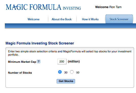
Now is a good time to mention that Joel Greenblatt has a website with a screener specifically for
the Magic Formula. The direct screener can be found
here. The screener
itself is very straightforward. You can enter in a market cap filter, and choose the number of
securities the screen should spit out.
We have some older data collected from Greenblatt's website, and will use one date to make a comparison between the official model and the one we have created. The original screen produced these results:
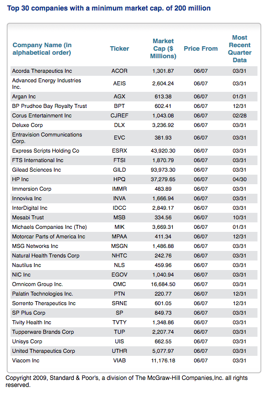
Running our own screen in the newly created Jupyter Notebook, on the same date as specified in the website data, our list of the Top 30 stocks are as follows:
| Official Website Screen | Our Quantopian Screen |
|---|---|
| ACOR | EVC |
| AEIS | AGX |
| AGX | NHTC |
| BPT | PINC |
| CJREF | PDLI |
| DLX | GME |
| EGOV | UTHR |
| ESRX | FTSI |
| EVC | PTN |
| FTSI | HPQ |
| GILD | AMCX |
| HPQ | OMC |
| IDCC | ZAGG |
| IMMR | PPC |
| INVA | INVA |
| MIK | MU |
| MPAA | SDI |
| MSB | KLIC |
| MSGN | BIG |
| NHTC | REGI |
| NLS | LPX |
| OMC | UIS |
| PTN | FL |
| SP | NRZ |
| SRNE | AYI |
| TUP | IMMR |
| TVTY | MTOR |
| UIS | IPG |
| UTHR | NLS |
| VIAB | ALSN |
The results of our screen did not completely replicate that of the screen produced by magicformulainvesting.com, and that is likely due to the fact that our calculations of tangible capital employed may have differed with Greenblatts. Nonetheless, almost half the securities from the official website made it into our screen, so we feel confident that our screen would produce securities with conceptually the characteristics of "cheap" and "good" as described in the book.
To Be Continued...